In a previous post, “The Great Unknown: Using the Statistics to Explore the Secret Depths of Unpublished Research,” I discussed one way a study can show something to be true when it's false, or vice versa.
If some nutrient or drug has a “true” biological effect, and we repeat many studies of the phenomenon, we would expect a handful of them to show a much greater effect than the real one and a handful of them to show a much lesser effect. In some instances, we might even expect to see the opposite effect turn up by random chance in a few studies. And if some nutrient or drug has no effect whatsoever, the bias against publishing negative results might leave us with a small handful of conflicting studies, some showing a positive effect and some showing a negative effect, but few if any showing the truth — no effect.
In my most recent post on gluten, I mentioned yet another way a study can show something to be true when it's false: regression to the mean. I also discussed regression to the mean in my 2006 article “Myth: One High Saturated Fat Meal Can Be Bad”, which was the basis for a much shorter letter I published in the Journal of the American College of Cardiology.
In this post I'll explain how this phenomenon can easily cause fake findings to be paraded around as true, and then use the real-life example of this ridiculous study making the absurd claim that statins cure vitamin D deficiency.
Regression to the mean is, in short, the tendency for really high values to fall towards the average value upon a second measurement and the equivalent tendency for really low values to rise towards the average value in the same way.This is incredibly common in research studies and if researchers do not randomly allocate subjects to control and treatment groups, or if they do but that randomization does not effectively produce equivalent characteristics within the two groups, or if the authors do not report the raw baseline values so that we as readers can verify that the randomization was effective, the study will be plagued by the vagaries of regression to the mean and its results will be completely uninterpretable.
If we are to read research critically, we should examine every study purporting to show a change in some measurement for regression to the mean. No stone should ever be left unturned.
Judy Simpson, then the Senior Lecturer in Statistics of the University of Sydney's Department of Public Health, wrote a 1995 article in the journal Statistics in Medicine in which she stated that “medical researchers need constant reminding of the effects of regression to the mean.”
Consider what the well respected textbook Statistics in Medical Research has to say:
In some studies of medical interventions, subjects are selected by preliminary screening tests as having high values of a relevant test measurement. For example, in studies of cholesterol-lowering agents, subjects may be selected as having serum cholesterol levels above some critical value, either on a single or on the mean of repeated determinations. On average, even with no effect of the agent under test, subsequent readings on the same subjects would tend to regress toward the mean. A significant reduction below the pretreatment values thus provides no convincing evidence of a treatment effect.”
Judy Simpson and David Newell, then an Emeritus Professor of Medical Statistics at the University of Sydney, wrote a 1990 review article in the Medical Journal of Australia on regression to the mean in which they recounted the following story:
[McDonald and colleagues] abstracted from 12,000 patient records the first and last measurements over a two-year period of 15 different biochemical variables, identified all those more than three standard deviations above the mean at the last measurement, and observed the value of the first measurement (this backwards manoeuvre avoids the possible effects of treatment). Every one of the 15 biochemical tests showed a reduction. For example, the mean total cholesterol concentration was 5.7 mmol/L, but when those with a last reading of 9.5 mmol/L or above were studied, the repeat measurement was on average 13% lower. (A similar result was obtained working forwards.) A treatment which lowered cholesterol by 13% should certainly not be ignored, but this was entirely a regression-to-the-mean effect. Essentially, with a cholesterol concentration as high as this there's nowhere (or hardly anywhere) else to go but down.”
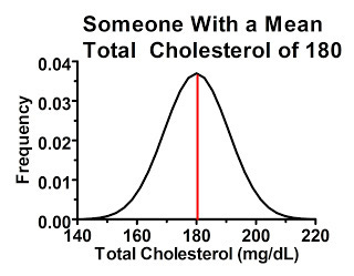
Why would this happen? There's actually considerable variation from measurement to measurement in many of these biochemical parameters, especially cholesterol, even when diet and lifestyle are held constant. Someone with a “true” or at least average total cholesterol of 180 mg/dL will tend to have values close to 180 when tested, but if you measure their cholesterol many times you'll probably get a distribution that looks something like this:
For the sake of simplicity, I'll give all these distributions a symmetrical bell-curve shape, where the average value is also the most common one. Things are often a little more complex than that in reality, but it suits our purpose here.
In the above graph, the red line represents the average cholesterol value. The range of possible values for this person is shown on the horizontal axis, and the higher we go on the vertical axis the more commonly we'll find that particular value. As we get further away from the red line, the person is less likely to get that particular value back on a cholesterol test, but as long as the value falls under the curve, it's possible.
Some of this variation is due to imperfect performance of the assay, but a great deal of it is due to true biological variation from hour to hour and from day to day and from season to season.
We can begin to understand regression to the mean by just considering this single individual. Since the values that are farthest from the mean are the least common, whenever we have a value far away from the mean on a first reading, the second reading will, on average, give a reading closer to the mean.
Now, let's say we are doing a study on people with “high cholesterol” and we define “high cholesterol” as over 200 mg/dL. Would this person be included? She might be, even though her cholesterol is actually 20 points lower than the cutoff. Why? Because just under 2.5 percent of the time her cholesterol measures in over 200 mg/dL!
Consequently, if we tested 100 people who's “true” cholesterol level is 180 mg/dL, two or three of them would likely have high enough cholesterol to be included in the study.
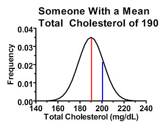
Now, let's consider a man who's average cholesterol is 190 mg/dL:
As you can see here, this guy has an even greater chance of being included in the study, even though his “true” or at least average cholesterol level is below the cutoff. The area under the curve to the right of the blue line indicates the probability of his cholesterol test coming back higher than 200 mg/dL. In fact, if we had 100 people who had cholesterol levels similar to this man, we would probably include at least 15 of them in the study.
Thus, if 200 mg/dL is our cutoff, we will essentially have two types of people within the study. The first type consists of people whose true mean cholesterol levels are lower than the cutoff, but we have included them because their measurement happened to be high for whatever reason when we screened them. The second type consists of people who really do have average cholesterol levels above the cutoff.
The first type of people will, on average, have lower cholesterol the next time they get it tested. This is because their average values are their most common values, and thus the laws of probability dictate that their most likely measurements will always be closer to the average than their last measurement. Thus while some of these people may have a similar or even higher cholesterol level when they are retested, the average of the group will be lower.
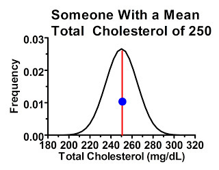
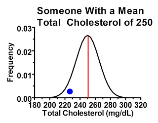
The second type of people were just as likely to have “high” readings compared to their own mean as they were to have “low” readings, because the cutoff point didn't select for one or another. Consider a subgroup of people within our study with average cholesterol levels of 250 mg/dL. The majority of these people, by the laws of probability, will have their first measurement similar to their mean, or at least hovering somewhere thereabouts, shown by the blue dot:
These people, by the laws of probability, are most likely to have a similar response in the next measurement providing we're not treating them with anything that effectively lowers cholesterol levels. Some of them may have lower or higher cholesterol levels next time, but they are no more likely to have lower ones than higher ones.
Less commonly, we might have people who had initial cholesterol readings higher than their own mean:
These people are overwhelmingly likely to have lower cholesterol levels the next time around.
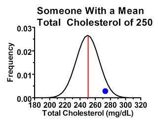
Yet cases like this are no more or common than the opposite:
These people are just as likely to have higher cholesterol next time around as the previous people were to have lower cholesterol the next time around. Thus, these extreme values tend to cancel each other out.
Since our cutoff was 200 mg/dL, however, there is no one on the “low” end of 180 or 190 mg/dL to cancel out the people on the high end of these means who were included in our study.
Thus, regardless of whether we treat anyone with an effective drug, the laws of probability dictate that simply because we had a cutoff that included only people with “high” cholesterol, the average cholesterol level will be lower at the end of the study.
The higher the cutoff, beyond a certain point, the more prominent this effect will be. This is because after a certain point we start encountering fewer and fewer people with such a high cholesterol. Thus, for really high cutoffs, we will have a higher proportion of borderline people whose true means are below the cutoff than we would have if we used a lower cutoff that was closer to the population mean.
It doesn't have to be a “high” cutoff point. Take this amusing example that Simpson offers as one of her favorites:
My favourite example of this is Brodribb and Humphrey's article on the effect of bran on oral-anal transit time. By dividing the subjects into three groups based on their initial transit times, they claim to show that those with the longest times are speeded up, while the fastest are slowed down. They conclude, “Bran seems to ‘normalise' transit times towards a mean of about 48 hours. While this phenomenon could merely be a regression towards the mean, we conclude that increasing the fibre intake does have a genuine physiological action in slowing fast transit times and accelerating slow transit times in patients with diverticular disease.”
In this case, there were two cutoff points that were used to define three groups: slow, medium, and fast. The slow got faster, the fast got slower, and the medium went nowhere. Big surprise, the two extremes regressed to the mean and the mean had nowhere to regress to. The authors found nothing but developed a convenient way to pretend they found something and somehow got their paper published.
What do we do about this? The answer is simple: we randomly allocate half our patients to a treatment group and half to a control group, though as we'll see below we still need to closely examine papers where this is done for regression to the mean.
Newell and Simpson explain:
In a controlled trial comparing a new treatment with a standard or a placebo treatment, with proper randomization regression to the mean should affect both treatment arms equally. The post-treatment difference in means gives the real benefit of new treatment, unbiased by regression to the mean. But if patients were selected on the basis of a high initial reading, the two mean improvements cannot themselves be interpreted as the treatment effect and the placebo effect, as both are likely to be inflated by regression to the mean.
There are three very important words: with proper randomization.
I would elaborate a bit to clarify that proper randomization is only proper if it is effective. Even if the investigators follow a proper randomization procedure, it is still possible for the randomization to fail to effectively make each group have similar characteristics at the beginning of the study. This failure can always happen but it is most likely in smaller studies.
As an example of ineffective randomization, the famous Wadsworth Veterans Administration Hospital Study randomized inpatients to eat foods cooked either in butter or vegetable oil, but there were twice as many heavy smokers and 60 percent more smokers in the butter group. Their finding that heart disease incidence (but not atherosclerosis) increased in the butter group thus does not provide convincing evidence that the butter was responsible. I described this study in the sidebar “Vegetable Oils and Heart Disease: A Closer Look” in my article “Precious Yet Perilous: Understanding the Essential Fatty Acids.”
But this is an example of confounding, not regression to the mean. Let's look first at a hypothetical example of how ineffective randomization can produce regression to the mean, and then at a few real-life examples, including the ridiculous statins-cure-vitamin-D-deficiency study.
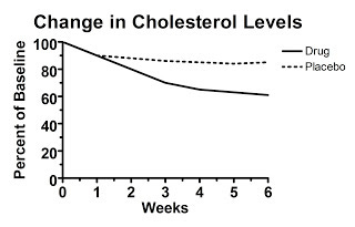
Let's say we look at a hypothetical study that presents data calculated as the change from baseline (that is, the change from the beginning of the study), but doesn't present the raw data. Here's figure one from this hypothetical study, claiming to show the treatment decreased cholesterol levels:
Here the starting value is set at 100 percent by definition. Over the six weeks, the average change from each person's initial value is shown. The authors report that the difference at six weeks is statistically significant.
Convinced?
You shouldn't be. Here's why. Somewhere behind this “change from baseline graph” lurks a graph of the raw data, but the authors didn't report it. What does the raw data look like?
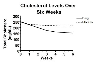
Well, it might look like this, which would be really convincing:
Here, the randomization was effective and the cholesterol levels were similar between the two groups at the beginning of the study. Some regression to the mean occurred in each group, but the difference between the groups at six weeks represents the true effect of the drug.
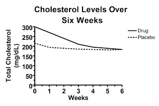
On the other hand, maybe the unpublished graph of the raw data looks like this:
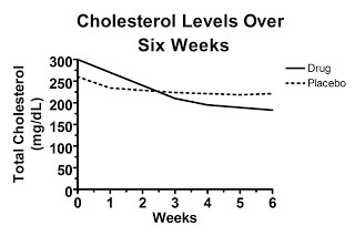
Here, the difference in change from baseline is exactly what was shown in the first graph, yet the baseline values between the two groups are so disparate at the beginning of the study that at six weeks average cholesterol levels are the same in each group! This suggests that the effect of the “drug” was entirely due to regression to the mean and in fact the drug is completely worthless. Nevertheless, you wouldn't have known it from “figure 1” because this graph wasn't published in our hypothetical paper.
Sometimes it's much more ambiguous. What if the unpublished graph of the raw data looks like this?
In this case, the cholesterol levels in the drug-treated group fell below the levels found in the placebo group, but the difference is similar to the difference between groups at the beginning of the study, which was clearly the result of random chance. If the difference at the end of the trial is statistically significant, that would suggest the drug was indeed effective, but the fact that random chance produced a similar difference at the beginning of the trial would certainly cast doubt on just how effective the drug really is.
This is why I have trouble taking the claim of the recent gluten study that gluten increased the severity of digestive symptoms seriously. They only reported “change from baseline” data, and we are left with no idea whether the unpublished graph of the raw data looks like our very convincing first pattern above, our thoroughly unconvincing second pattern, or our ambiguous third pattern.
Unfortunately, the authors did not even discuss this possibility. The words “regression to the mean” do not appear in the paper.
By contrast, the authors of the one-meal-high-in-saturated-fat-will-kill-you study did include a discussion of this possibility, probably because the editor or the reviewers required them to:
Although the differences in FMD, arterial diameter, and flow at baseline between the groups were nonsignificant, it is possible that “regression to the mean” may have contributed to some of the FMD reduction observed after consumption of the saturated fat (although all analyses were “blinded” to meal assignment and timing).”
They said this because they tried to show that saturated fat harms vascular function by showing that vascular function decreased after the saturated fat meal but not after the polyunsaturated fat meal.
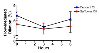
Let's take a look at their data:
Hmm, what's that difference at time zero? All the participants consumed both meals, one on each of two different occasions separated by a month. The investigators randomized some participants to get coconut oil first and others to get safflower oil first, but obviously the randomization wasn't very effective at producing similar vascular function at baseline.
In fact, vascular function was better in the saturated fat group through the entire study. Are we to believe that the “decline” in vascular function after the saturated fat meal is attributable to anything other than regression to the mean?
If we accept what Newell and Simpson wrote above, that “the post-treatment difference in means gives the real benefit of new treatment, unbiased by regression to the mean,” then we would have to conclude that the type of fat had no effect at all.
Now, for our finale, let's take a look at the preposterous claim that statins cure vitamin D deficiency.
The authors treated 83 patients who were hospitalized for an acute coronary syndrome with Lipitor. Most of the patients (ninety percent) had been hospitalized for a heart attack while ten percent had stable angina. Most of the subjects were also on various blood pressure drugs.
Most of the patients (75 percent) had vitamin D deficiency at the start of the study, defined as 25(OH)D under 20 ng/mL, and the mean 25(OH)D level was 17 ng/mL.
Right away, what can we spot? The subjects have low vitamin D. If Lipitor has no effect, what's likely to happen? The vitamin D levels are likely to increase, and the proportion of people classified as deficient is likely to decline, because of regression to the mean.
This regression to the mean could occur not only because of random fluctuations, but even because of their disease state. What if a recent heart attack causes a transient decrease in 25(OH)D? After a year, each person's vitamin D status is likely to return to normal.
Now, every good study has subjects randomly allocated to a control group, right? Well, not this study. Here the control group was “73 hypertensive patients not receiving treatment with statins.”
This, of course, cannot in any remote way be considered a “control group” because these people are not a random sample of the initial subject population, and because they have an entirely different disease condition!
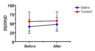
Nevertheless, let's look at their data:
Well, as in the saturated fat study, the supposed treatment effect is never able to overcome the large difference at baseline, even though in this case we don't even have a true randomized control. Where is the evidence that this effect was anything other than regression to the mean? Nowhere to be found.
There are ways that investigators can attempt to statistically adjust for regression to the mean, but usually investigators are trying to prove their point rather than undermine it, so you don't see this terribly often. It is generally up to the critical reader to look for regression to the mean.
Here are a few tips for identifying this phenomenon:
Always make sure that the treatment not only produces a change from baseline, but a true difference by the end of the study compared to a randomized control group.
Beware of any study that claims a stronger effect in the people who were in the worst condition at the start of the study. This could be a true biological phenomenon, but regression to the mean is too obvious an explanation to be dismissed.
Ensure that the values of interest were very similar at baseline between both groups. If there is a large difference, it could contribute to regression to the mean even if it's not statistically significant.
If the study has no control group, or doesn't report the baseline values, be skeptical. Be very, very skeptical.
Well, that's what I would do anyway.
And thus we see that many published research findings are false. Some of these false findings exist because we would inevitably expect by the laws of probability for a small handful of well conducted, thoroughly reported, and appropriately interpreted studies to uncover apparent truths that are really false simply by random chance. This emphasizes the need to look at the totality of the data. Some will be false because of regression to the mean. This emphasizes the need to critically evaluate the data in each study.
Then, after slicing and dicing a biological hypothesis from many different angles and attempting to reconcile all the data into a big picture, we come ever more close to the intrinsically elusive biological truth we are in pursuit of.


